The following example compares two MDS solutions for the well-known Ekman colour-perception data, derived from two different scaling programs. These data, which have frequently been used to illustrate non-metric scaling methods, are based on paired comparisons of stimuli in the form of light displays accross the visible spectrum, and are essentially two-dimensional. The solutions compared here, although originally superficially different in appearance, are shown to be practically identical in the first two dimensions, with minor differences occurring only in the third dimension, which has been included here for demonstration purposes. The third dimension can consequently be eliminated.
This example also illustrates a useful feature of multidimensional scaling conventions, namely that configurations are regarded as equivalent if they remain the same subject to what are here labelled "Similarity Transformations", which preserve the orderings of the distances between the points of which they are made up.
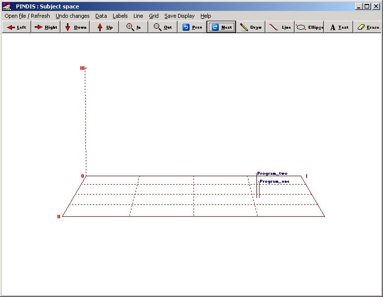
The 'subject space' looks like this :
Clicking on shows the following detailed information for the PINDIS analysis. This confirms the visual impression above, that the two solutions compared are practically identical.
                     ------------------

      Two scalings of the EKMAN data

 Fit of Centroid Configuration
  0.011047
  0.011047

 Centroid configuration
    1        W434   -0.1103   -0.2149   -0.0606
    2        W445   -0.1336   -0.1980   -0.0337
    3        W465   -0.2596   -0.1139   -0.0091
    4        W472   -0.2732   -0.0877    0.0290
    5        W490   -0.2553    0.0726   -0.0097
    6        W504   -0.1794    0.2087   -0.0026
    7        W537   -0.0893    0.2443   -0.0886
    8        W555   -0.0542    0.2685    0.0090
    9        W584    0.1684    0.1666    0.0913
   10        W600    0.2348    0.0818   -0.0210
   11        W610    0.2660   -0.0339   -0.0172
   12        W628    0.2564   -0.0975    0.0098
   13        W651    0.2237   -0.1408    0.0117
   14        W674    0.2057   -0.1557    0.0919


 ****  Perspective Origins  ****
 Subject
    1     -0.1606     -0.2959      1.3429
    2      0.0935      0.3574     -1.1140

 ****  Analytic Solutions for Individual Configurations   ****

 ****  Configuration for Subject   1  ****
 **** Program one

 1)  Similarity Transformations

  Normed scalar for unconditional weights:  1.000000

    1       W434   -0.1153   -0.2246   -0.0203
    2       W445   -0.1322   -0.2022    0.0181
    3       W465   -0.2582   -0.1100   -0.0423
    4       W472   -0.2720   -0.0860    0.0154
    5       W490   -0.2537    0.0735   -0.0430
    6       W504   -0.1821    0.2123   -0.0276
    7       W537   -0.0845    0.2515   -0.0706
    8       W555   -0.0554    0.2622    0.0501
    9       W584    0.1648    0.1619    0.0907
   10       W600    0.2310    0.0802   -0.0202
   11       W610    0.2718   -0.0362   -0.0180
   12       W628    0.2590   -0.0930    0.0025
   13       W651    0.2200   -0.1369   -0.0231
   14       W674    0.2069   -0.1526    0.0883

 Fit of subject to centroid/hypothesis  ---  S(Z,X) =  0.988953

 2)  Dimensional-weighting Transformations

 Dimensional Weights:
           1.0003      1.0025      0.7870
 Dimensional Correlations:
           0.9999      0.9996      0.8223

 Fit   ---  S(ZW,X)=  0.990200

 3)  Perspective Models - Vector Weighting

 Translation of Individual Configuration:
          -0.0386      0.0313      0.1126
 Stimuli:                Vector Weights:      Vector Cosines:
   1       W434              1.0907              0.9916
   2       W445              1.0845              0.9863
   3       W465              0.9743              0.9946
   4       W472              0.9928              0.9992
   5       W490              0.9807              0.9951
   6       W504              1.0011              0.9973
   7       W537              1.0313              0.9983
   8       W555              1.0336              0.9931
   9       W584              0.9738              0.9999
  10       W600              0.9644              0.9999
  11       W610              0.9928              0.9997
  12       W628              0.9648              0.9992
  13       W651              0.8868              0.9915
  14       W674              0.9694              0.9999

 Fit   ---   S(VZ,X)=  0.992072

 4) Joint Weighting Solution

 Dimensional Weights:
           1.0055      1.0075      0.8054
 Vector Weights:
   1       W434        1.0138
   2       W445        0.9836
   3       W465        0.9874
   4       W472        0.9866
   5       W490        0.9938
   6       W504        1.0105
   7       W537        1.0107
   8       W555        0.9748
   9       W584        0.9922
  10       W600        0.9790
  11       W610        1.0176
  12       W628        0.9968
  13       W651        0.9698
  14       W674        1.0057

 Fit   ---   S(VZW,X)=  0.990303

 ****  Configuration for Subject   2  ****
 **** Program two

 1)  Similarity Transformations

  Normed scalar for unconditional weights:  1.004231

    1       W434   -0.1041   -0.2028   -0.1004
    2       W445   -0.1335   -0.1916   -0.0851
    3       W465   -0.2582   -0.1165    0.0241
    4       W472   -0.2714   -0.0884    0.0422
    5       W490   -0.2540    0.0709    0.0237
    6       W504   -0.1747    0.2028    0.0224
    7       W537   -0.0931    0.2344   -0.1057
    8       W555   -0.0524    0.2719   -0.0321
    9       W584    0.1701    0.1694    0.0908
   10       W600    0.2360    0.0824   -0.0217
   11       W610    0.2573   -0.0312   -0.0162
   12       W628    0.2509   -0.1010    0.0171
   13       W651    0.2250   -0.1431    0.0463
   14       W674    0.2022   -0.1570    0.0945

 Fit of subject to centroid/hypothesis  ---  S(Z,X) =  0.988953

 2)  Dimensional-weighting Transformations

 Dimensional Weights:
           0.9884      0.9864      1.2016
 Dimensional Correlations:
           0.9999      0.9996      0.9109

 Fit   ---  S(ZW,X)=  0.990200

 3)  Perspective Models - Vector Weighting

 Translation of Individual Configuration:
          -0.0301      0.0329      0.1144
 Stimuli:                Vector Weights:      Vector Cosines:
   1       W434              0.8787              0.9832
   2       W445              0.8866              0.9753
   3       W465              1.0153              0.9965
   4       W472              0.9965              0.9996
   5       W490              1.0188              0.9957
   6       W504              1.0021              0.9968
   7       W537              0.9764              0.9988
   8       W555              0.9708              0.9936
   9       W584              1.0221              1.0000
  10       W600              1.0283              1.0000
  11       W610              0.9879              0.9994
  12       W628              1.0108              0.9994
  13       W651              1.0833              0.9945
  14       W674              1.0051              1.0000

 Fit   ---   S(VZ,X)=  0.992053

 4) Joint Weighting Solution

 Dimensional Weights:
           0.9956      0.9902      1.1956
 Vector Weights:
   1       W434        0.9883
   2       W445        1.0172
   3       W465        0.9994
   4       W472        1.0026
   5       W490        0.9923
   6       W504        0.9787
   7       W537        0.9810
   8       W555        1.0145
   9       W584        0.9872
  10       W600        1.0089
  11       W610        0.9697
  12       W628        0.9917
  13       W651        1.0215
  14       W674        0.9771

 Fit   ---   S(VZW,X)=  0.990256

 Normalized Dimension Weights
 Subject  Communality          1         2         3
    1        0.9902         0.7701    0.6146    0.1397
    2        0.9902         0.7609    0.6047    0.2134
   Mean
 Communality 0.9902         0.5860    0.3717    0.0325


      ---  Table of Subject Communalities for PINDIS Transformations ---

                                 Transformation
   Z,X[i] ZW[i],X[i]  Z[i]W[i],X[i]  V[i]Z,X[i]  V[i]Z[i],X[i]  V[i]ZW[i],X[i]
 ------------------------------------------------------------------------------

   1  0.99    0.99        0.99          0.99          1.00          0.99
   2  0.99    0.99        0.99          0.99          1.00          0.99

 Mean 0.99    0.99        0.99          0.99          1.00          0.99

 ------------------------------------------------------------------------------
          * 0.0 means that particular PINDIS transformation was not used.
For further information about these procedures, see the
references included with these notes.